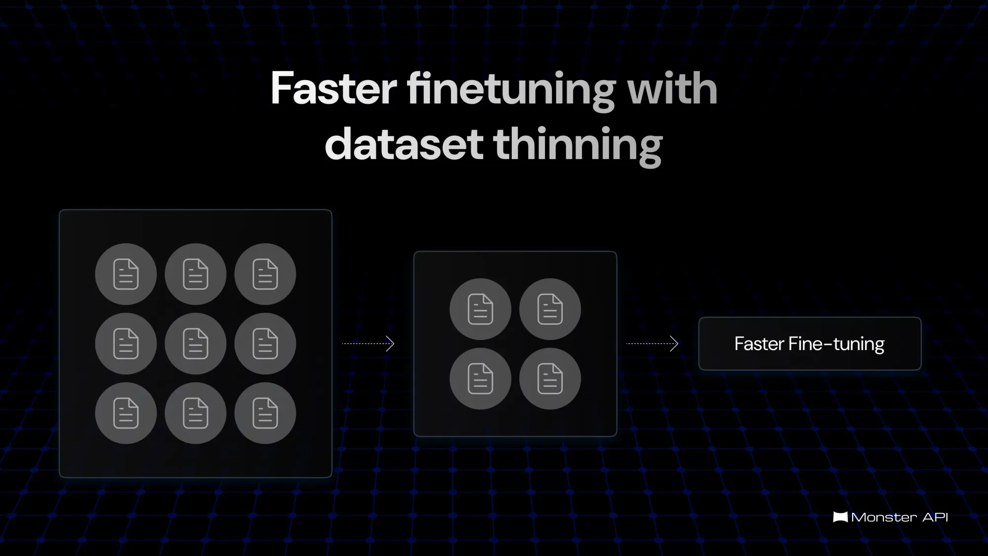
Dataset Thinning for faster fine-tuning of LLMs

Fine-tuning large language models (LLMs) on a massive dataset can be a significantly time-intensive process. The more extensive the dataset, the longer it takes for the model to process each batch of data, which slows down the overall training time. This can result in extended periods required for model convergence, making it difficult to iterate quickly and refine the model for specific tasks.

Additionally, the computational load increases with the size of the data, leading to higher resource consumption and potentially longer wait times between training cycles. This slowdown in fine-tuning is a common challenge when dealing with enormous datasets.

Importance of Dataset in Fine-tuning.

One of the questions that is often left unanswered while dealing with datasets to fine-tune models is how good the data is? Often people think that the more data they have for a task the better they can fine-tune a model that is often the quality of data is wrongly associated with the quantity.

An ideal dataset contains no clusters in it. Clusters are associated with redundancy in the data. Training with a lot of redundant data can often result in a model that is overly biased towards the clusters present in the dataset. These kinds of overfitting is difficult to identify and can degrade the performance of the models.

Clustering the dataset can provide some valuable insights into the underlying redundancy and can potentially alleviate overfitting. One of the ideal clustering algorithms to use here will be DBSCAN. DBSCAN is a density-based clustering algorithm that automatically clusters the dataset without requiring the user to specify the number of clusters to form explicitly.

One other useful thing with DBSCAN is that it also identifies noise points in the dataset alongside clusters. Essentially noise points are unique data points in the dataset and we don’t want to remove them.

Clustering a Dataset & Thinning Redundancies

Now let us see how we can cluster a dataset and thin down the redundancies in it using just DBSCAN and Sentence Transformers.

Let us first install the required packages sk-learn for DBSCAN sentence-transformers for embedding matplotlib datasets and pandas to support.

!pip install scikit-learn sentence_transformers matplotlib datasets pandas

Next step is to import the dataset and select the column that represents the input to the model.

from datasets import load_dataset
texts = load_dataset("RaagulQB/Tested-143k-Python-Alpaca-llama-formatted", split="train")["instruction"]

Next step is to choose an embedding model to embed our dataset column. There are a lot of models available within sentence transformers the ‘all-MiniLM-L6-v2’ is the fastest.

from sentence_transformers import SentenceTransformer
model = SentenceTransformer('all-MiniLM-L6-v2',device='cuda')

import tqdm
embeddings = []
for text in tqdm.tqdm(texts):
  embeddings.append(model.encode(text))

Once embedding is finished we can cluster the embeddings using DBSCAN

from sklearn.cluster import DBSCAN
import numpy as np

eps = 0.5
min_samples = 5

dbscan = DBSCAN(eps=eps, min_samples=min_samples)
dbscan.fit(embeddings)


cluster_assignments = dbscan.labels_

If we print out the cluster assignment we will get an ouput something like this

array([-1, -1, -1, ..., -1, -1, -1])

here all the -1 represents that the point is a noise point we can plot the entire distribution and visualize the distribution of data among clusters.

cluster_dict = {}
for idx, label in enumerate(cluster_assignments):
    if label not in cluster_dict:
        cluster_dict[label] = []
    cluster_dict[label].append(texts[idx])

import matplotlib.pyplot as plt
# Assuming cluster_assignments is a numpy array containing the cluster labels from DBSCAN
cluster_labels, counts = np.unique(cluster_assignments, return_counts=True)

plt.figure(figsize=(12, 8))
plt.barh(cluster_labels, counts, color='skyblue')
plt.xlabel('Number of Examples')
plt.ylabel('Cluster Labels')
plt.title('Number of Examples per Cluster')
plt.gca().invert_yaxis()  # Invert y-axis to have clusters in ascending order
plt.grid(axis='x')

# Show the plot with better spacing
plt.tight_layout()
plt.show()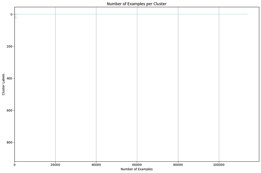

In our case most of the data points were noise and we had 800+ smaller clusters of redundant data. Next step is to reduce the redundant data. Here we have simply reduced out 50% of all non-noise clusters randomly.

import random
# New dictionary to store the thinned clusters
thinned_cluster_dict = {}

for label, texts in cluster_dict.items():
  if label == -1:
    thinned_cluster_dict[label] = texts
    continue
  thinned_size = max(1, len(texts) // 2)  # Ensure at least one item is selected
  thinned_texts = random.sample(texts, thinned_size)
  thinned_cluster_dict[label] = thinned_texts

# Output the thinned cluster dictionary
for label, texts in thinned_cluster_dict.items():
    print(f"Cluster {label}:")
    print(len(texts))

To verify the effectiveness of thinning out the dataset we fine-tuned Gemma-2–2B on both the complete and thinned datasets and the training and validation losses are presented below.

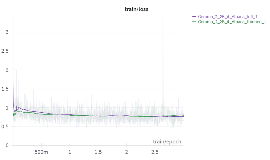
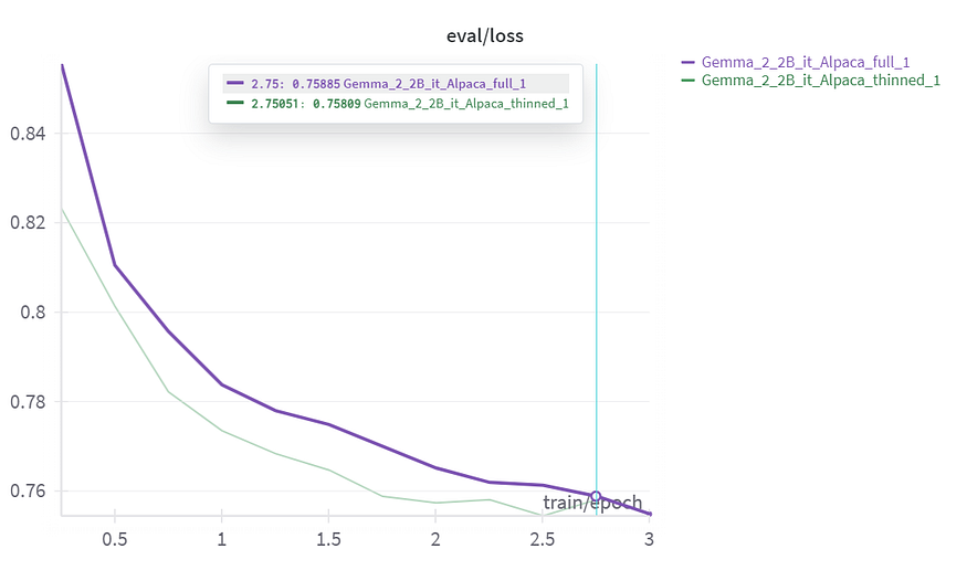
The training loss of both the models does not differ much and converges to almost the same point it essentially proves that the pruned off points does not contribute much to the learning. And from the validation loss we can understand that pruning off repetitive points contributes to the loss by consistently maintaining a better validation loss compared to the model trained on the full dataset.

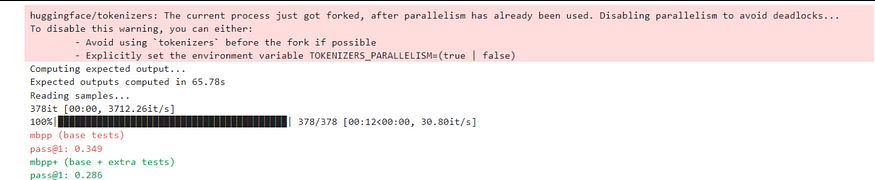
further to evaluate the training we benchmarked the fine-tuned model on MBPP and it was able to outperform Gemma2–2B-it. (Base model benchmarks are referred from the Google’s technical report)

Summing Up

Overall, one can use this clustering as a metric to understand the quality of the dataset and potentially reduce the size of the dataset. Further experimentations can be done by taking various datasets various embeddings and various thinning strategies. (For example, one can decide to thin down proportional to the size of clusters).